Sensor ingestion, windowing, and the difference between fast and realtime
6.1 The puzzle
In August 2020, a wildfire ignited in scrub near a network of automated environmental sensors in southern California. The sensor network was working. Thermistors and smoke particulate detectors registered anomalous readings within minutes of ignition. The readings were transmitted successfully to a data collection endpoint.
The alert arrived forty minutes later.
Forty minutes was long enough that suppression resources had already been dispatched — not from the sensor network, but from a phone call made by a hiker who saw smoke. By the time the automated alert fired, incident commanders were already staging equipment. The sensor system, which cost considerably more than the phone, contributed nothing to the initial response.
What went wrong? Not the sensors. Not the transmission. The ingestion pipeline was batch-processing. Every hour, it pulled the previous hour’s readings from the collection endpoint, computed summary statistics, and compared those statistics against thresholds. At 11:00, it processed 10:00–11:00 and found no anomalies. At 12:00, it processed 11:00–12:00 and raised an alert for elevated temperature and particulates beginning at 11:22.
The fire started at 11:22. The alert arrived at 12:00.
This is not a story about broken software. The batch pipeline was doing exactly what it was designed to do. The failure was architectural: the latency requirement of the application — detect a fire within minutes — was never translated into a latency constraint on the data pipeline. Batch processing was chosen because it is simpler to operate, and nobody asked whether “simpler” was compatible with the use case.
The question this chapter addresses is: what would a different data architecture look like, and how do you decide when you need it?
6.2 Batch vs streaming: a latency decision
The distinction between batch and streaming is not primarily a technology choice. It is a latency requirement that determines which technology is appropriate.
Batch processing treats data as a bounded dataset: collect records until some condition is met (time elapsed, record count reached, file received), then process the entire set. Latency is bounded below by the batch interval. A one-hour batch cannot produce an alert in less than one hour from the triggering event, even if processing itself takes one second.
Stream processing treats data as an unbounded sequence of events arriving over time. Records are processed as they arrive, or within a short configurable window. Latency is bounded by propagation delay, processing time, and window size — potentially seconds or milliseconds.
The tradeoff is operational complexity. A batch pipeline is a script that runs on a schedule. A stream processing system requires persistent processes, state management, failure recovery, and careful reasoning about what happens when messages arrive late or out of order. You take on that complexity only when the latency requirement demands it.
Most spatial data applications are not realtime. An overnight batch pipeline that updates a dashboard of aggregated sensor readings is entirely appropriate for planning or reporting use cases. The wildfire scenario is different: response time to an ignition event is measured in minutes, and a forty-minute pipeline latency is a failure mode, not a design choice.
6.2.1 Event time vs processing time
When a sensor emits a reading, two timestamps are relevant.
Event time is when the measurement was taken — the timestamp embedded in the reading by the sensor or the collection system at the moment of capture.
Processing time is when the record arrives at the processing system.
In a well-functioning local network these are nearly identical. In a sensor network with intermittent connectivity — a field device reporting via cellular, a buoy with a satellite uplink, a vehicle that uploads its track when it returns to a docking station — event time and processing time can differ by minutes, hours, or days.
This matters because you almost always want to aggregate by event time, not processing time. A five-minute window of temperature readings should contain readings from those five minutes, not readings that happened to arrive during those five minutes. If a sensor was offline for an hour and uploaded a backlog when reconnected, those readings should be placed in the correct historical windows, not dumped into the current window because that is when they arrived.
This is the late data problem, and it is endemic to spatial sensor networks. The processing system needs a mechanism for handling records that arrive after the window they belong to has already been computed. That mechanism is the watermark.
6.2.2 Watermarks
A watermark is the processing system’s estimate of how far behind the leading edge of event time the stream has fallen. If the watermark is at T − 5 minutes, the system is asserting: all events with event time before T − 5 have arrived. Any window ending before T − 5 can be finalised.
Setting the watermark too aggressively (small lag) causes the system to close windows before all data has arrived, dropping late records. Setting it too conservatively (large lag) delays results, because windows cannot be emitted until the watermark passes their end time.
For a sensor network with known connectivity patterns, the watermark can be tuned empirically: measure the distribution of (processing time − event time) across your devices, set the watermark lag at the 95th or 99th percentile of that distribution, and accept that a small fraction of records will arrive late and be dropped or redirected to a separate late-data handler.
For the wildfire network: if sensor readings are transmitted every 30 seconds over a reliable local radio link, a 60-second watermark lag is conservative and allows near-realtime window evaluation. If the same sensors report via cellular with occasional 10-minute gaps, a 15-minute watermark lag is more appropriate — but now the latency guarantee is 15 minutes, which may or may not satisfy the application requirement.
The architectural decision is: what latency can the use case tolerate, and does the watermark policy deliver that latency given the connectivity characteristics of the sensor network?
6.3 Kafka: persistent logs for sensor streams
Apache Kafka is the most widely deployed system for high-throughput event streaming. It is worth understanding how it works before deciding whether you need it — many spatial systems do not need Kafka’s throughput, but the conceptual model it imposes (a persistent, replayable log) is useful regardless of which system you use.
6.3.1 Topics, partitions, and offsets
A Kafka topic is a named, ordered sequence of records. Topics are analogous to database tables, but append-only: you can write records and read records, but you cannot update or delete them. Records are retained for a configurable duration (often days or weeks).
A topic is divided into partitions. Each partition is an independent ordered log. Records within a partition are strictly ordered; records across partitions are not. Partitioning is the source of Kafka’s throughput: multiple producers can write to different partitions simultaneously, and multiple consumers can read from different partitions simultaneously, with no coordination overhead between them.
For a spatial sensor network, a natural partitioning key is sensor ID or geographic region. All readings from sensor 47 go to the same partition in the same order they were produced. A consumer reading that partition sees a strictly ordered sequence of readings from that sensor, which simplifies state management for per-sensor computations.
Every record in a partition has an offset — a monotonically increasing integer assigned by the broker. A consumer tracks the offset of the last record it processed. If the consumer crashes and restarts, it resumes from its last committed offset. This makes Kafka consumers stateless with respect to position: the broker remembers where each consumer group left off.
The offset mechanism also makes replay possible. If a processing bug is discovered, you can reset a consumer group’s offset to an earlier point in the log and reprocess historical records. For a sensor network, this means you can re-derive aggregates, correct for a faulty calibration factor, or backfill a downstream database after a schema change — without re-querying the sensors.
6.3.2 Consumer groups
A consumer group is a set of consumer processes that collectively read a topic. Kafka assigns each partition to exactly one consumer in the group. If you have 12 partitions and 4 consumers, each consumer reads 3 partitions. If one consumer dies, its partitions are reassigned to the survivors. If you add consumers, partitions are rebalanced.
The throughput implication: you can scale consumption by adding consumers, up to the number of partitions. A topic with 1 partition cannot benefit from more than 1 consumer in a group. For a sensor network expecting growth, provision more partitions than you currently need.
6.3.3 Minimal producer and consumer in Python
The following is a static example — it requires a running Kafka broker and is not executable in the browser. It shows the structural pattern, not a production-ready implementation.
# requires: pip install kafka-python# requires: a running Kafka broker at localhost:9092# topic 'sensor-readings' must exist (or auto-create must be enabled)from kafka import KafkaProducer, KafkaConsumerimport jsonimport timeimport random# --- Producer: emit synthetic sensor readings ---producer = KafkaProducer( bootstrap_servers=["localhost:9092"], value_serializer=lambda v: json.dumps(v).encode("utf-8"), key_serializer=lambda k: k.encode("utf-8"),)SENSOR_IDS = [f"sensor-{i:03d}"for i inrange(10)]def emit_reading(sensor_id: str) ->None: reading = {"sensor_id": sensor_id,"event_time": time.time(),"temperature_c": round(20.0+ random.gauss(0, 2.0), 2),"smoke_ug_m3": round(max(0, random.gauss(5, 1.5)), 2), } producer.send( topic="sensor-readings", key=sensor_id, # partition key: all readings from one sensor value=reading, # serialised to JSON bytes )# Emit one reading per sensor per secondwhileTrue:for sid in SENSOR_IDS: emit_reading(sid) producer.flush() time.sleep(1.0)
# --- Consumer: read and print readings from the topic ---consumer = KafkaConsumer("sensor-readings", bootstrap_servers=["localhost:9092"], group_id="alert-processor", # consumer group auto_offset_reset="latest", # start from newest records value_deserializer=lambda b: json.loads(b.decode("utf-8")), key_deserializer=lambda b: b.decode("utf-8") if b elseNone,)ALERT_THRESHOLD_TEMP_C =45.0ALERT_THRESHOLD_SMOKE =50.0for message in consumer: reading = message.value partition = message.partition offset = message.offsetif (reading["temperature_c"] > ALERT_THRESHOLD_TEMP_C or reading["smoke_ug_m3"] > ALERT_THRESHOLD_SMOKE):print(f"ALERT partition={partition} offset={offset}"f" sensor={reading['sensor_id']}"f" temp={reading['temperature_c']}°C"f" smoke={reading['smoke_ug_m3']} µg/m³" )
The key structural points: the producer uses the sensor ID as the partition key, ensuring ordered delivery per sensor. The consumer commits offsets per consumer group, enabling crash recovery. Threshold logic applied to individual records here is the simplest possible alerting pattern — the next section covers window-based aggregation, which is more appropriate for sensor noise.
6.4 MQTT: for sensor-scale IoT
Kafka is designed for high-throughput, durable log storage. It runs on a JVM, requires significant memory and disk, and has operational overhead that is not justified for small sensor networks or constrained devices.
MQTT (Message Queuing Telemetry Transport) is a publish-subscribe protocol designed for constrained environments. An MQTT broker has a much lighter footprint than a Kafka cluster. MQTT clients run on microcontrollers with kilobytes of RAM. The protocol was originally designed for oil pipeline monitoring over satellite links with high latency and low bandwidth.
6.4.1 Broker, topics, and QoS levels
An MQTT broker (Mosquitto is the common open-source implementation) mediates all communication. Publishers send messages to topic strings; subscribers receive messages matching their topic subscriptions. MQTT topic strings are hierarchical and support wildcards:
sensors/wildfire/region-north/sensor-047/temperature — a specific reading type from a specific sensor
sensors/wildfire/region-north/+/temperature — temperature from all sensors in region-north (+ matches one level)
sensors/wildfire/# — everything under the wildfire prefix (# matches any number of levels)
Quality of Service (QoS) levels control delivery semantics:
QoS 0 (at most once): fire-and-forget. The broker does not acknowledge receipt. Fastest, but messages may be dropped on unreliable links.
QoS 1 (at least once): the broker acknowledges receipt; the publisher retransmits until acknowledged. Messages are delivered but may be duplicated.
QoS 2 (exactly once): a four-way handshake ensures exactly one delivery. Slowest, highest overhead. Appropriate only when deduplication at the application layer is impractical.
For environmental sensors where a dropped reading is acceptable but a duplicate reading would double-count toward an aggregate, QoS 1 with application-layer deduplication is a reasonable choice. For billing or regulatory reporting, QoS 2.
MQTT does not persist a replayable log in the way Kafka does. Most brokers support retained messages (the broker keeps the last message on a topic and delivers it immediately to new subscribers) but not full history. For that reason, MQTT is typically used as the ingestion layer — sensors publish to an MQTT broker, and a bridge process subscribes and writes to a more durable store (Kafka, TimescaleDB, or a flat file archive).
# --- Subscriber: receive and process readings ---def on_connect(client, userdata, flags, rc):if rc ==0:# subscribe to all temperature readings in region-north client.subscribe("sensors/wildfire/region-north/+/temperature", qos=1)print("Subscribed")else:print(f"Connection failed: rc={rc}")def on_message(client, userdata, msg): payload = json.loads(msg.payload.decode("utf-8"))print(f"topic={msg.topic}"f" sensor={payload['sensor_id']}"f" temp={payload['temperature_c']}°C" )sub_client = mqtt.Client(client_id="alert-subscriber")sub_client.on_connect = on_connectsub_client.on_message = on_messagesub_client.connect(BROKER_HOST, BROKER_PORT, keepalive=60)sub_client.loop_forever()
MQTT is appropriate when sensors are numerous and constrained, network links are unreliable or low-bandwidth, and you do not need Kafka’s durable replay capability at the sensor layer. Pair it with a bridge to a durable store if replay or long-term retention matters.
6.5 Windowing: time-based aggregation
Individual sensor readings are noisy. A single temperature spike could be sensor noise, an insect landing on the thermistor, a momentary reflection of sunlight. Acting on individual readings produces false alarms. The wildfire sensor scenario requires detecting a sustained elevation in temperature and smoke — a signal that persists across multiple readings, not a single outlier.
Windowing is the mechanism. Instead of processing individual records, the stream processor groups records into time-based windows and computes aggregates over each window. The aggregate (mean, max, count above threshold) is more stable than the raw reading and more appropriate for alerting.
6.5.1 Tumbling windows
A tumbling window has a fixed size and does not overlap. All windows cover the same duration; each record falls in exactly one window. A 5-minute tumbling window at 10:00 covers 10:00–10:05. The next window covers 10:05–10:10. Records do not appear in both.
Tumbling windows are appropriate for aggregates you report on a regular schedule: “the mean temperature in each 5-minute interval.” They have a fixed latency: results are available at most one window period after the triggering event.
6.5.2 Sliding windows
A sliding window has a fixed size and a step smaller than the window size, so consecutive windows overlap. A 5-minute window with a 1-minute step produces a new result every minute, each covering the previous 5 minutes. Every record appears in multiple windows (up to window_size / step).
Sliding windows are appropriate for continuous anomaly detection: you want to know the current 5-minute mean at any point in time, not just at 5-minute boundaries. The tradeoff is computational: each record is processed once per window it participates in.
6.5.3 Session windows
A session window groups records by a gap of inactivity. If records arrive within a threshold gap of each other, they are in the same session. If a gap exceeds the threshold, the window closes and a new one opens.
Session windows are appropriate for event-driven patterns where activity comes in bursts: a vehicle’s GPS track while it is moving (session) vs stationary (gap), or a sensor that reports only when conditions change rather than on a fixed schedule.
6.5.4 The latency-accuracy tradeoff
Shorter windows detect events faster but are noisier. Longer windows are more stable but slower. A 1-minute window detects a fire onset roughly 1 minute after it starts — but is sensitive to individual noisy readings. A 10-minute window is more robust to noise but imposes a 10-minute detection latency.
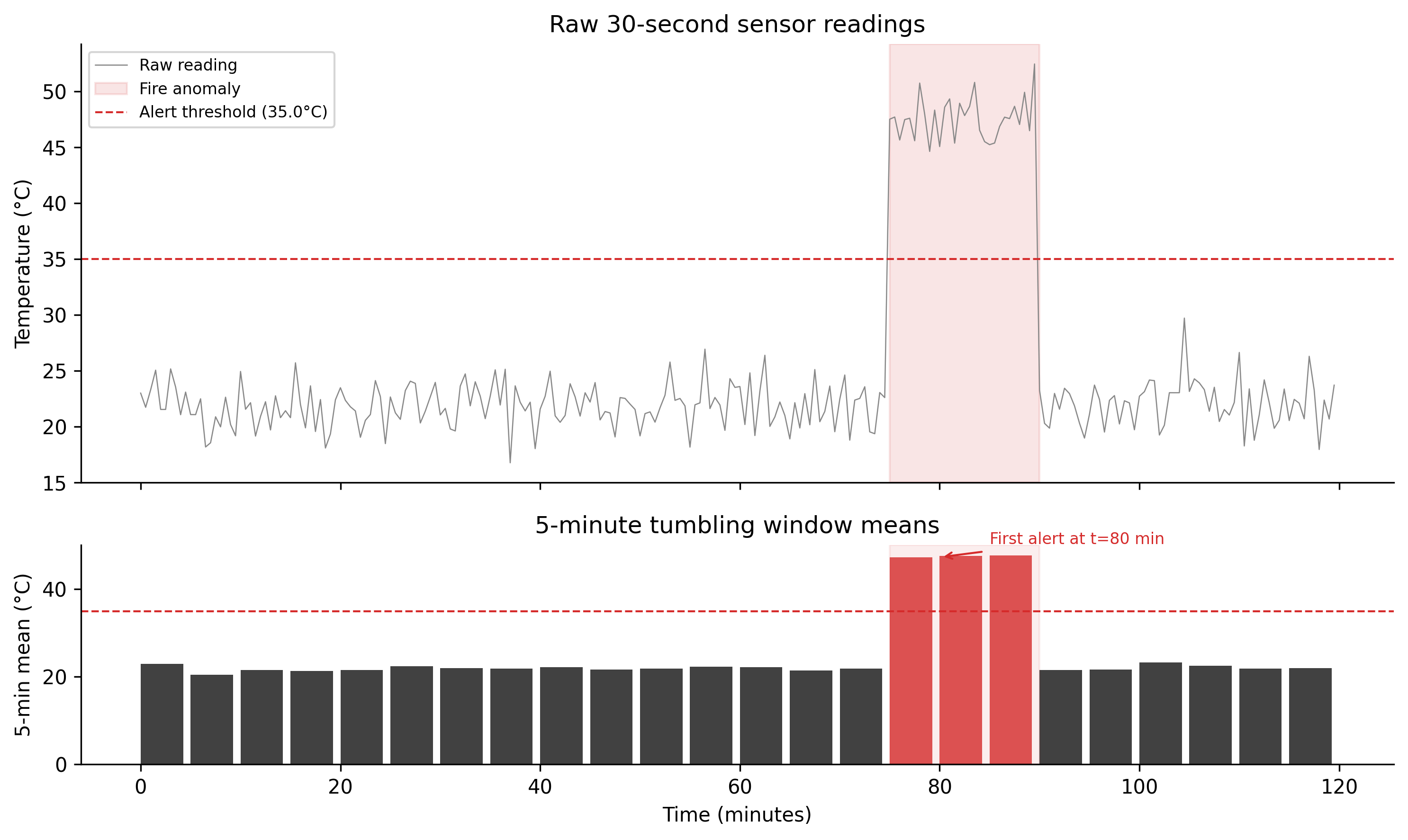
For the wildfire scenario: if sensor noise has standard deviation 2°C and fire onset produces a sustained 20°C elevation, a 5-minute tumbling window with a threshold set at 10°C above baseline should detect the fire within one window period (5 minutes) with low false alarm rate. That is a meaningful improvement over a 60-minute batch.
Figure 6.1: Figure 5.1. Windowed sensor aggregation. Top panel: raw 30-second temperature readings for a simulated 2-hour period. Gaussian noise (σ = 2°C) overlays a baseline of 22°C. A fire anomaly is injected at t = 75 minutes, raising temperature by 25°C for 15 minutes. Bottom panel: 5-minute tumbling window means. The anomaly window mean exceeds the alert threshold (35°C) within the first full window after ignition, at t = 80 minutes — 5 minutes after onset. Compare this with the 60-minute batch interval that produced the original failure.
6.6 Backpressure
A stream processing system has two rates: the rate at which the producer emits records, and the rate at which the consumer processes them. When the consumer is slower than the producer, the queue between them grows. If the queue is unbounded and the imbalance persists, the system runs out of memory and crashes. If the queue is bounded, the system must decide what to do when it fills: drop new records, block the producer, or signal the producer to slow down.
That signal is backpressure — the consumer communicating its capacity back to the producer.
Kafka’s pull model handles this naturally. Consumers request records at their own pace; the broker does not push. If a consumer is slow, it falls behind — its lag (distance between its current offset and the partition’s latest offset) grows. The records are retained on the broker until the consumer catches up or the retention window expires. The producer is never blocked by consumer slowness. The cost is latency: a slow consumer introduces delay between record production and processing, and if it falls far enough behind, records may expire before they are consumed.
Push models (MQTT with QoS 0, many HTTP webhook systems) have no natural backpressure. The broker sends records as fast as they arrive. A slow consumer either drops records or buffers them in memory until the buffer overflows.
For spatial sensor networks, the typical failure mode is a sudden burst of readings — a sensor network coming online after a maintenance window, a data backfill after an outage, or a sudden increase in sampling frequency during an event. Kafka’s pull model absorbs these bursts without producer-side impact. The consumer lag increases temporarily; it drains as the consumer processes the backlog. The key operational metric is consumer lag: if lag trends upward continuously, the consumer cannot keep up and you need to either increase consumer parallelism (add consumers up to the partition count) or reduce per-record processing cost.
The buffer stock analogy is exact: the Kafka partition log is a buffer stock between producer and consumer. Its level (lag) rises when the inflow rate (producer throughput) exceeds the outflow rate (consumer throughput) and falls when the consumer is faster. A well-managed system maintains lag near zero during normal operation and recovers quickly after bursts.
6.7 What to try
TipWhat to try
Change WINDOW_SIZE from 5 to 1 minute. Does the alert fire sooner? What happens to the false positive rate during the baseline period before the anomaly? There is a real tradeoff here, not a free lunch.
Raise ANOMALY_MAGNITUDE_C to 5 and lower it to 2. At what magnitude does the windowed mean reliably exceed the threshold? What does this imply about the sensitivity of the alert threshold relative to the noise level?
Increase NOISE_STD_C to 8. What happens to the number of window means that exceed the threshold during the baseline period? How would you adjust the threshold to maintain a low false positive rate?
# --- Try changing these parameters ---DURATION_MINUTES =120# total simulation length (minutes)WINDOW_SIZE =5# tumbling window size (minutes, try 1 or 10)NOISE_STD_C =2.0# sensor noise std dev (°C, try 8.0)ANOMALY_MAGNITUDE_C =25.0# fire temperature elevation (°C, try 5.0)ANOMALY_TIME =75# fire start (minutes into simulation)ALERT_THRESHOLD_C =35.0# alert threshold (°C)import numpy as npimport matplotlib.pyplot as pltnp.random.seed(42)BASELINE_TEMP_C =22.0SAMPLE_INTERVAL_S =30ANOMALY_DURATION_MIN =15samples_total =int(DURATION_MINUTES *60/ SAMPLE_INTERVAL_S)t_s = np.arange(samples_total) * SAMPLE_INTERVAL_St_m = t_s /60.0temperature = BASELINE_TEMP_C + np.random.normal(0, NOISE_STD_C, samples_total)anomaly_mask = (t_m >= ANOMALY_TIME) & (t_m < ANOMALY_TIME + ANOMALY_DURATION_MIN)temperature[anomaly_mask] += ANOMALY_MAGNITUDE_Csamples_per_window =max(1, int(WINDOW_SIZE *60/ SAMPLE_INTERVAL_S))n_windows = samples_total // samples_per_windowwindow_means = np.array([ temperature[i * samples_per_window:(i +1) * samples_per_window].mean()for i inrange(n_windows)])window_starts = np.array([ t_m[i * samples_per_window] for i inrange(n_windows)])alert_windows = window_means > ALERT_THRESHOLD_Cfirst_alert = np.argmax(alert_windows) if alert_windows.any() elseNonefig, (ax1, ax2) = plt.subplots(2, 1, figsize=(10, 5), sharex=True, gridspec_kw={"height_ratios": [2, 1]})ax1.plot(t_m, temperature, color="#888888", linewidth=0.5, label="Raw")ax1.axvspan(ANOMALY_TIME, ANOMALY_TIME + ANOMALY_DURATION_MIN, alpha=0.12, color="#d52a2a", label="Fire")ax1.axhline(ALERT_THRESHOLD_C, color="#d52a2a", linewidth=1, linestyle="--", label=f"Threshold {ALERT_THRESHOLD_C}°C")ax1.set_ylabel("Temp (°C)")ax1.legend(fontsize=7, loc="upper left")ax1.spines["top"].set_visible(False)ax1.spines["right"].set_visible(False)bar_colors = ["#d52a2a"if a else"#333333"for a in alert_windows]ax2.bar(window_starts, window_means, width=WINDOW_SIZE *0.85, align="edge", color=bar_colors, alpha=0.8)ax2.axhline(ALERT_THRESHOLD_C, color="#d52a2a", linewidth=1, linestyle="--")ax2.axvspan(ANOMALY_TIME, ANOMALY_TIME + ANOMALY_DURATION_MIN, alpha=0.08, color="#d52a2a")ax2.set_ylabel(f"{WINDOW_SIZE}-min mean (°C)")ax2.set_xlabel("Time (minutes)")ax2.spines["top"].set_visible(False)ax2.spines["right"].set_visible(False)plt.tight_layout()plt.show()n_false_positives =int(alert_windows[:int(ANOMALY_TIME / WINDOW_SIZE)].sum())if first_alert isnotNone: alert_at = window_starts[first_alert] + WINDOW_SIZEprint(f"First alert at t = {alert_at:.1f} min "f"(fire started at t = {ANOMALY_TIME} min)")else:print("No alert raised.")print(f"False positives before anomaly: {n_false_positives}")print(f"Window size: {WINDOW_SIZE} min | "f"Noise std: {NOISE_STD_C}°C | "f"Anomaly magnitude: {ANOMALY_MAGNITUDE_C}°C")
6.8 Exercises
5.1 — Latency budget
The wildfire sensor network in the opening scenario used a 60-minute batch interval. A wildfire suppression team requires a response time of 8 minutes from ignition to alert dispatch.
Sketch the complete latency budget from ignition event to alert dispatch, including: sensor sampling interval, transmission lag, ingestion processing, windowing lag, alert evaluation, and notification delivery. Assign realistic values to each component.
What is the maximum allowable windowing lag if all other components are fixed at your estimated values?
If the cellular link introduces up to 3 minutes of transmission lag, what watermark policy is appropriate?
5.2 — Partition key selection
A sensor network covers 500 sensors across 20 geographic regions. You are designing a Kafka topic with 20 partitions.
Compare the following partition key strategies: (i) sensor ID, (ii) geographic region, (iii) hash of sensor ID mod 20. What are the ordering guarantees each provides? What are the throughput implications?
A downstream consumer computes per-region aggregates. Which partition key strategy makes this consumer simplest to implement? Why?
A new requirement arrives: the consumer must also compute cross-region correlations. Does your answer to (b) change?
5.3 — Watermark policy
You have telemetry from 200 field sensors. Connectivity statistics over the past 30 days show: - 80% of readings arrive within 10 seconds of event time - 95% arrive within 2 minutes - 99% arrive within 8 minutes - The remaining 1% can arrive up to 6 hours late (sensors that were offline overnight)
You are computing 5-minute tumbling windows for a realtime dashboard. What watermark lag do you recommend? What fraction of records will be late-dropped?
You need a separate daily summary with complete data. How would you handle the 6-hour-late records? Describe an architecture that serves both use cases.
5.4 — Backpressure under load
A Kafka consumer group has 4 consumers reading a topic with 12 partitions. Normal consumer lag is under 500 records. During a sensor backfill event, lag spikes to 200,000 records.
How long will it take to drain the backlog if the consumer processes 1,000 records per second and the producer emits 800 records per second?
The operations team proposes adding 8 more consumers to drain faster. Will this help? What is the maximum number of consumers that can usefully read from a 12-partition topic?
An alternative proposal is to increase per-consumer parallelism by using async processing within each consumer. What risk does this introduce, and how would you mitigate it?
6.9 Build this
Design and implement a Kafka-based sensor ingestion system with stream processing. The system has two components: a producer that emits synthetic sensor readings, and a Faust stream processor that computes 5-minute spatial aggregates.
Producer (producer.py): emits synthetic temperature and smoke readings for 50 sensors across 5 geographic regions. Each reading has sensor ID, region, event timestamp, temperature, and smoke concentration. Readings are emitted at configurable intervals with Gaussian noise and an optional injected anomaly.
Stream processor (processor.py): uses Faust (a Python stream processing library built on Kafka) to compute 5-minute tumbling window means per region, emit an alert when any window mean exceeds a threshold, and write region-level aggregates to a separate Kafka topic.
# producer.py# requires: pip install kafka-python# requires: Kafka broker at localhost:9092from kafka import KafkaProducerimport json, time, random, mathBROKER = ["localhost:9092"]TOPIC ="spatial-sensor-readings"N_SENSORS =50REGIONS = ["north", "south", "east", "west", "central"]EMIT_INTERVAL_S =30NOISE_STD_C =2.0SMOKE_NOISE =1.5SEED =42# Each sensor is assigned a region deterministicallySENSOR_REGION = {f"sensor-{i:03d}": REGIONS[i %len(REGIONS)]for i inrange(N_SENSORS)}producer = KafkaProducer( bootstrap_servers=BROKER, value_serializer=lambda v: json.dumps(v).encode(), key_serializer=lambda k: k.encode(),)random.seed(SEED)def make_reading(sensor_id: str, t: float) ->dict: region = SENSOR_REGION[sensor_id]# Inject a fire anomaly into the "north" region between t=3600 and t=4500 anomaly =25.0if (region =="north"and3600<= t %7200<=4500) else0.0return {"sensor_id": sensor_id,"region": region,"event_time": t,"temperature_c": round(22.0+ random.gauss(0, NOISE_STD_C) + anomaly, 2),"smoke_ug_m3": round(max(0, random.gauss(5, SMOKE_NOISE) + anomaly *0.8), 2), }start = time.time()print(f"Producer started. Emitting {N_SENSORS} sensors every {EMIT_INTERVAL_S}s.")whileTrue: t = time.time() - startfor sid in SENSOR_REGION: reading = make_reading(sid, t) producer.send(TOPIC, key=reading["region"], value=reading) producer.flush() time.sleep(EMIT_INTERVAL_S)
To run: start a Kafka broker, then in two terminals: python producer.py and faust -A processor worker -l info. The aggregate topic receives one message per region per window period. Monitor consumer lag with kafka-consumer-groups.sh --bootstrap-server localhost:9092 --describe --group spatial-aggregator.